Linear regression in R: how to read the output

Fit a linear regression in R with lm() and interpret every part of the summary — coefficients, p-values, R-squared and residuals — plus a tidy table with broom.

lm() is one of the most-used functions in R, and its summary() packs a lot into a small space. Here’s how to read every piece. (Predicting a binary outcome instead? See logistic regression.)

Fit the model

We’ll predict fuel economy (mpg) from weight and horsepower using the built-in mtcars:

fit <- lm(mpg ~ wt + hp, data = mtcars)
summary(fit)

Call:
lm(formula = mpg ~ wt + hp, data = mtcars)

Residuals:
   Min     1Q Median     3Q    Max 
-3.941 -1.600 -0.182  1.050  5.854 

Coefficients:
            Estimate Std. Error t value Pr(>|t|)    
(Intercept) 37.22727    1.59879  23.285  < 2e-16 ***
wt          -3.87783    0.63273  -6.129 1.12e-06 ***
hp          -0.03177    0.00903  -3.519  0.00145 ** 
---
Signif. codes:  0 '***' 0.001 '**' 0.01 '*' 0.05 '.' 0.1 ' ' 1

Residual standard error: 2.593 on 29 degrees of freedom
Multiple R-squared:  0.8268,    Adjusted R-squared:  0.8148 
F-statistic: 69.21 on 2 and 29 DF,  p-value: 9.109e-12

Reading the summary

• Coefficients (Estimate) — the change in mpg for a one-unit increase in that predictor, holding the others constant. Here each 1,000 lb of weight (wt) costs several mpg.
• Pr(>|t|) — the p-value for “this coefficient is zero.” Small means the predictor carries information beyond the others.
• Multiple R-squared — the share of variance in mpg explained by the model. Adjusted R-squared penalises extra predictors and is the fairer figure to compare models.
• Residual standard error — the typical size of the model’s prediction errors, in mpg.

A tidy table

broom turns the model into data frames that are easy to report or plot:

library(broom)
tidy(fit, conf.int = TRUE)   # coefficients + 95% CIs

# A tibble: 3 × 7
  term        estimate std.error statistic  p.value conf.low conf.high
  <chr>          <dbl>     <dbl>     <dbl>    <dbl>    <dbl>     <dbl>
1 (Intercept)  37.2      1.60        23.3  2.57e-20  34.0      40.5   
2 wt           -3.88     0.633       -6.13 1.12e- 6  -5.17     -2.58  
3 hp           -0.0318   0.00903     -3.52 1.45e- 3  -0.0502   -0.0133

glance(fit)                  # model-level stats

# A tibble: 1 × 12
  r.squared adj.r.squared sigma statistic  p.value    df logLik   AIC   BIC
      <dbl>         <dbl> <dbl>     <dbl>    <dbl> <dbl>  <dbl> <dbl> <dbl>
1     0.827         0.815  2.59      69.2 9.11e-12     2  -74.3  157.  163.
# ℹ 3 more variables: deviance <dbl>, df.residual <int>, nobs <int>

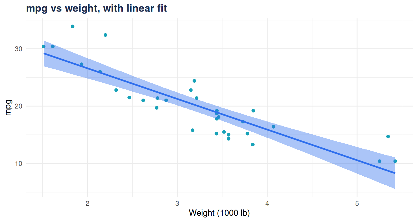
library(ggplot2)
ggplot(mtcars, aes(wt, mpg)) +
  geom_point(colour = "#17a2b8") +
  geom_smooth(method = "lm", se = TRUE, colour = "#2f6fed", fill = "#2f6fed22") +
  labs(title = "mpg vs weight, with linear fit", x = "Weight (1000 lb)", y = "mpg") +
  theme_minimal(base_family = "sans") +
  theme(plot.title = element_text(face = "bold", colour = "#1b2a4a"))

Figure 1

Don’t skip the diagnostics

A regression is only trustworthy if its assumptions hold. Run plot(fit) to check linearity, constant variance and normal residuals before you interpret a single coefficient.

---

Regression with confounders, interactions or a report to produce? That’s our statistical analysis service.