Sample size calculation in R: t-tests, proportions and correlations

How to compute the sample size you need in R with power.t.test and power.prop.test — the four quantities that trade off, worked examples, and a power curve you can adapt.

The question every study should answer before collecting a single data point: how many participants do I need? Too few and a real effect slips through; too many and you waste time and money. R has this built in — no extra packages required. (Prefer to just get a number? Use our sample size calculator.)

The four quantities

Sample size, effect size, significance level (α) and power are locked together — fix any three and the fourth follows. Usually we fix α = 0.05, power = 0.80, state the effect we care about, and solve for n.

# two-sample t-test: how many per group to detect d = 0.5?
power.t.test(delta = 0.5, sd = 1, power = 0.80,
             sig.level = 0.05, type = "two.sample")

     Two-sample t test power calculation 

              n = 63.76576
          delta = 0.5
             sd = 1
      sig.level = 0.05
          power = 0.8
    alternative = two.sided

NOTE: n is number in *each* group

The delta/sd ratio here is Cohen’s d. R uses the exact noncentral-t distribution, so this is the reference answer other calculators approximate.

Proportions and correlations

# comparing two proportions
power.prop.test(p1 = 0.50, p2 = 0.30, power = 0.80, sig.level = 0.05)$n

[1] 92.99884

# correlation via Fisher's z (base R)
n_for_r <- function(r, power = 0.8, alpha = 0.05) {
  C <- 0.5 * log((1 + r) / (1 - r))
  ceiling(((qnorm(1 - alpha/2) + qnorm(power)) / C)^2 + 3)
}
n_for_r(0.30)

[1] 85

See the trade-off

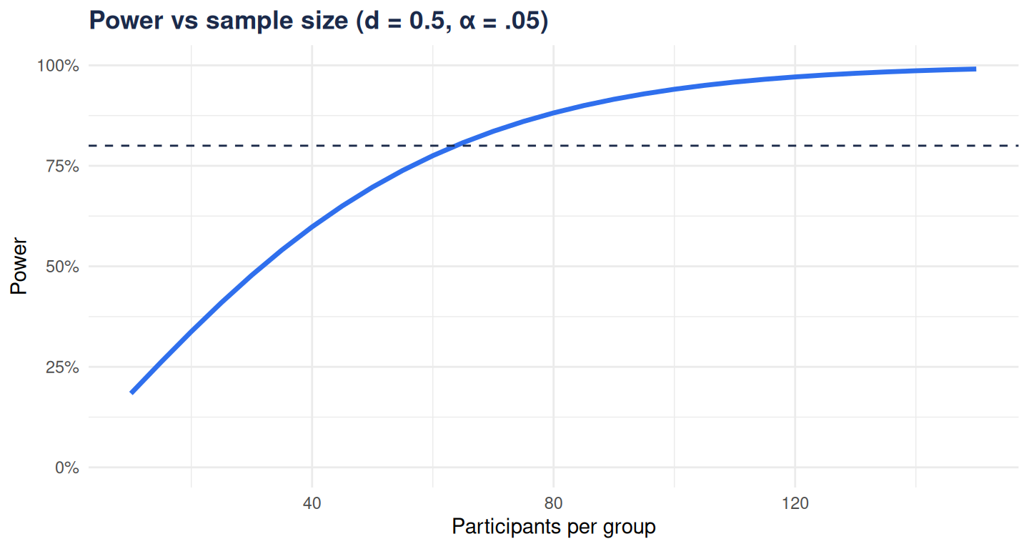
The most useful output isn’t one number — it’s the curve showing how power grows with sample size:

library(ggplot2)
ns <- seq(10, 150, 5)
pw <- sapply(ns, function(n)
  power.t.test(n = n, delta = 0.5, sd = 1, sig.level = 0.05)$power)

ggplot(data.frame(ns, pw), aes(ns, pw)) +
  geom_line(colour = "#2f6fed", linewidth = 1.2) +
  geom_hline(yintercept = 0.8, linetype = 2, colour = "#1b2a4a") +
  scale_y_continuous(labels = scales::percent, limits = c(0, 1)) +
  labs(title = "Power vs sample size (d = 0.5, α = .05)",
       x = "Participants per group", y = "Power") +
  theme_minimal(base_family = "sans") +
  theme(plot.title = element_text(face = "bold", colour = "#1b2a4a"))

Figure 1

The one rule

Base your effect size on prior evidence or the smallest difference that would matter — never on what gives a convenient n. When in doubt, compute across a range and report the sensitivity.

---

Need a sample size defended in writing for an ethics board or grant? That’s our statistical analysis service. Or try the calculator.